Since we announced our collaboration with the World Bank and more partners to create the Open Traffic platform, we’ve been busy. We’ve shared two technical previews of the OSMLR linear referencing system. Now we’re sharing more about how we’re using Mapzen Map Matching to “snap” GPS-derived locations to OSMLR segments, and how we’re using a data-driven approach to evaluate and improve the algorithms.
In the last blog post on Mapzen’s map-matching service, we showed you how Mapzen uses synthetic GPS data to validate the results of our map-matching algorithm. This time around, we’ll dive a bit deeper into the internals of the algorithm itself to see how we can use our validation metrics to fine-tune the map-matching parameters. First, we’ll determine parameter values that should work well given any level of GPS noise and frequency. Next, we’ll show how to optimize the parameters even further when we know more about the location and characteristics of a GPS data provider.
This post is also available as a Python notebook with code samples!
Parameter Definitions
The Open Traffic Reporter map-matching service is based on the Hidden Markov Model (HMM) design of Newson and Krumm (2009). HMM’s define a class of models that utilize a directed graph structure to represent the probability of observing a particular sequence of events—or in our case, a particular sequence of road segments that defines a route. For our purposes, it is enough to know that HMM’s are, in general, governed by two probability distributions which we’ve parameterized using σz and β, respectively. If, however, you are interested in a more detailed explanation of how HMM’s work in the context of map-matching, please see the excellent map-matching primer written by Mapzen’s own routing experts.
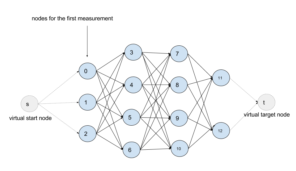
The graph structure of an HMM for an example route, from Mapzen’s map-matching algorithms primer
The parameter σz appears in the equation below which expresses the likelihood of recording a GPS measurement zt from road segment ri as the following Gaussian probability density function (PDF):
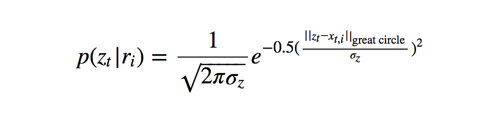
where xt,i is the point on road segment ri nearest the measurement zt at time t.
In practice, σz can be thought of as an estimate of the standard deviation of GPS noise.
The more we trust our measurements, the lower the value of our σz should be.
Newson and Krumm (2009) derive σz from the median absolute deviation over their dataset, arriving at a value of 4.07, which we have adopted as our default parameter value.
The β parameter comes from the following exponential PDF:

where dt is the difference between the great circle distance and route-traveled distance between time t and t+1. We use an exponential PDF to define this probability because Newson and Krumm (2009) found that for two successive GPS measurements, the differences in length between the “great circle” distance (i.e. “as-the-crow-flies” distances) and the corresponding route-traveled distance are exponentially distributed:
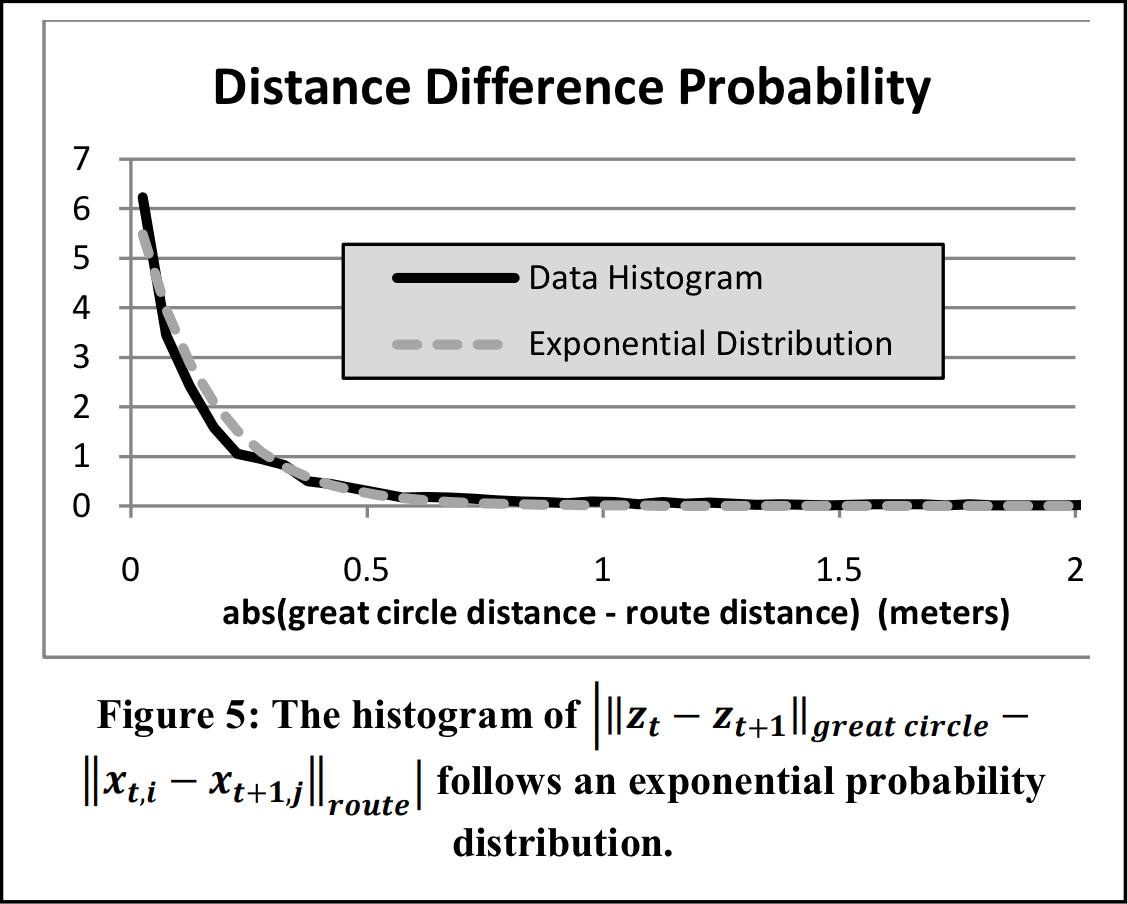
In this context, β can be thought of as the expected difference between great circle distances and route distance traveled, or in other words, the degree of circuitousness of our expected routes.
We have adopted a β of 3 as our default parameter value.
Grid search
Although we can empirically derive our parameter values using the equations above, we can also just search the space of feasible parameter values to find the ones that give the best results. This is a common machine learning approach for algorithm optimization, typically referred to as a grid search or parameter sweep. Grid search requires a reliable scoring mechanism in order to compare results. Lucky for us, we already implemented a number of these in our exploration of validation metrics.
Since we have to pick one to use in the grid search, we’ll stick with Newson and Krumm’s distance-based error metric for now, since it appears most frequently in the literature. Let’s take a quick look back at what those errors looked like over our set of validation data:
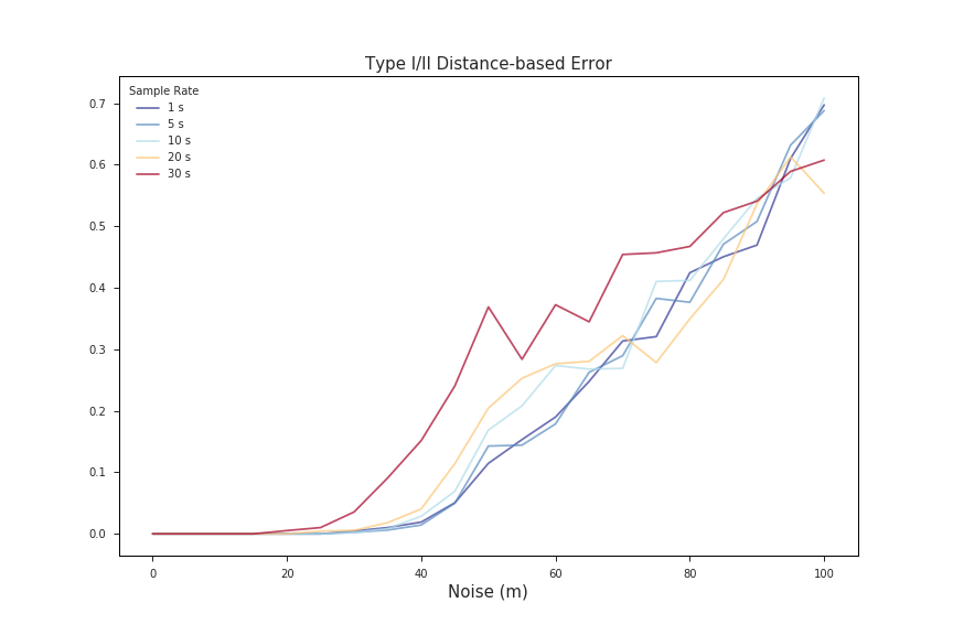
Clearly the quality of our data, by way of GPS noise and sample rate, has a huge impact on match error. Taking that into consideration, in addition to searching over the feasible space of β’s and σz’s, we’ll want to iterate over different noise levels and sample rates so that we can optimize our map-matching regardless of the quality of the data we receive.
Define the search space
Because this grid search takes place in such high dimensional space
noise levels
noiseLevels = np.linspace(0, 100, 6)   # in meters
sampleRates = [1, 5, 10, 20, 30]   # in seconds
betas = np.linspace(0.5, 10, 20)   # no units
sigmas = np.linspace(0.5, 10, 20)    # no units
Search and score
We’ve wrapped the entire grid search code into the grid_search_hmm_params() function since the internals are pretty messy. Behind the scenes, though, grid_search_hmm_params() proceeds as follows:
for route in routes:
    for beta in betas:
        for sigma in sigmas:
            for noise in noiseLevels:
                for rate in sampleRates:
                    i) simulate gps
                    ii) match routes
                    iii) score the route
    write scores to a route-specific file
Depending on the dimensions of your search space, grid search can be a long and arduous process. In our case, on a 2015 MacBook Pro, it seems to take ~1 min. per route for a given noise level and sample rate. With the configuration specified above, that works out to roughly 30 minutes per route. While this runtime does indeed seem a bit absurd, the beauty of grid search is that if you properly define your search space, you should really only need to do it once.
val.grid_search_hmm_params(
    cityName, routeList, sampleRates, noiseLevels, betas, sigmas)
Get optimal parameters
Combine the scores for all routes
Because of the slow runtime, grid_search_hmm_params() saves its results incrementally in route-specific files. We must first recombine them into a single master dataframe so that we can query, plot, and otherwise manipulate the data all together:
frame = val.mergeCsvsToDataFrame(
    dataDir='../data/sf200/', matchString='*.csv')
The first five rows of the combined dataframe:
frame.head()
| sample_rate | noise | beta | sigma_z | score | |
|---|---|---|---|---|---|
| 0 | 1 | 0.0 | 0.5 | 0.5 | 0.000000 |
| 1 | 5 | 0.0 | 0.5 | 0.5 | 0.000000 |
| 2 | 10 | 0.0 | 0.5 | 0.5 | 0.000000 |
| 3 | 20 | 0.0 | 0.5 | 0.5 | 0.219928 |
| 4 | 30 | 0.0 | 0.5 | 0.5 | 0.219928 |
Visualize scores
Now we visually can assess the parameter scores to check for global optima or tease out any other patterns that might persist across the various dimensions of our grid search. The get_param_scores() function will also return a dictionary of optimal parameter values corresponding to each one of the subplots below:
paramDict = val.get_param_scores(
    frame, sampleRates, noiseLevels, betas, sigmas, plot=True)
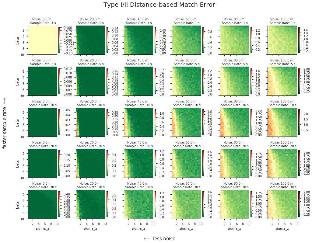
In our case there does appear to be a “global” trend of decreasing error toward the upper right quadrants of our plots, which correspond to higher σz’s and lower β’s. If we wanted to optimize our parameters across all sample rates and noise levels at once, the results suggest that our optimal parameters would lie at the maximum σz and minimum β values of our search space. This is an interesting finding, and not entirely satistfying, since it is typically unwise to pick parameter values at the limits of your search space—who knows what may lie on the other side? Although this could be evidence that we didn’t cast a wide enough net in our parameter sweep, there is reason to believe that it might not be worthwhile to search any further:
- Focusing specifically at the plots in the 0 - 40 m range of noise, it’s pretty clear that expanding the range of feasible parameter values wouldn’t do any good. You can’t get much better than 0 error, and our plots in this range are already dominated by dark green. We can obtain optimal results by picking parameters anywhere in this dark green zone.
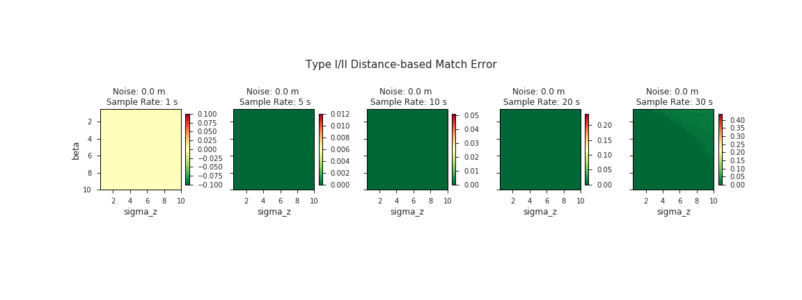
Behold small multiples: while the full grid above shows the sample rate along the y-axis, here we’ve transposed the data with sample rate running along the x-axis and we collapsed the other axis into a GIF.
We expect most of our data to be within this bottom half of the range of noise levels we tested. According to the Institute of Navigation, GPS-enabled smartphones can typically achieve an accuracy of ~5 m. Even taking into consideration the fact that most Open Traffic data providers will be operating in dense urban environments where GPS is notoriously inaccurate, we still expect to be operating primarily in the realm sub-60 m of noise. It is likely not to our advantage to tune our algorithm parameters to optimize for the worst-case scenario.
In the range of noiser data (> 60 m), although there is very little dark green in the plots, there is also no evidence to suggest that we should expect to do any better by increasing our search space. In fact, our inuition about the limitations of map-matching with extremely noisy GPS data tells us that the opposite is probably true. There is only so much we can expect the algorithm to do with data once its positional accuracy is less than the length of a standard city block.
Performing a grid search over this many different parameters is extremely slow.
Taking these ideas into consideration, it is clear that expanding our search space would yield diminishing returns. Instead, we’ll use the results we’ve already got to make a more informed decision about how we want to fine-tune our parameters. In the next section, we’ll implement such an approach for one hypothetical transportation network company (TNC).
Case study: “A-OK Rides”
Consider a hypothetical TNC called A-OK Rides. A-OK Rides happens to be based in London, and nearly 90% of A-OK trips either start or end in the city’s central business district. In order to conserve bandwidth and processing power, the A-OK app only collects GPS measurements from A-OK drivers every 20 seconds. In this case study, we’ll see how to use this contextual information about our partner’s service territory and anticipated data quality in order to improve our match results.
cityName = 'London'
routes = val.get_POI_routes_by_length(
     cityName, minRouteLength=1, maxRouteLength=5, numRoutes=100, apiKey=gmapsKey)
Since we know that almost 90% of our GPS data will be generated from within an area dominated by skyscrapers and other forms of dense urban development, this is a case where we actually do want to optimize for noisier data. As such, we will perform our parameter sweep over routes generated with 60 m of noise:
noiseLevels = [60] # meters
Similarly, since A-OK only collects data every 20 seconds, we can make sure we are only optimizing for data generated at this frequency:
sampleRates = [20] # seconds
We’ll search for our optimal β and σz values over the same space as before:
betas = np.linspace(0.5, 10, 20)
sigmas = np.linspace(0.5, 10, 20)
val.grid_search_hmm_params(
    cityName, routes[24:], sampleRates, noiseLevels, betas, sigmas)
And retrieve the parameter values that gave us the generated the lowest matching error:
paramDf = val.mergeCsvsToDataFrame(
    dataDir='../data/', matchString="London*.csv")
paramDict = val.get_param_scores(
    paramDf, sampleRates, noiseLevels, betas, sigmas, plot=False)
beta, sigma = val.get_optimal_params(
    paramDict, sampleRateStr='20', noiseLevelStr='60')
print('Sigma: {0} // Beta: {1}'.format(sigma, beta))
We can now generate new routes, score them using out optimal parameter values, and compare the match errors to what we would have obtained using our default parameters. This will tell us how much our parameter optimization has improved the performance of our map-matching algorithm.
newRoutes = val.get_POI_routes_by_length(
    cityName, 1, 5, 100, gmapsKey)
tunedDf, _, _ = val.get_route_metrics(
    cityName, newRoutes, sampleRates, noiseLevels,sigmaZ=sigma, beta=beta, saveResults=False)
defaultDf, _, _ = val.get_route_metrics(cityName, newRoutes, sampleRates, noiseLevels, saveResults=False)
val.plot_err_before_after_optimization(defaultDf, tunedDf)
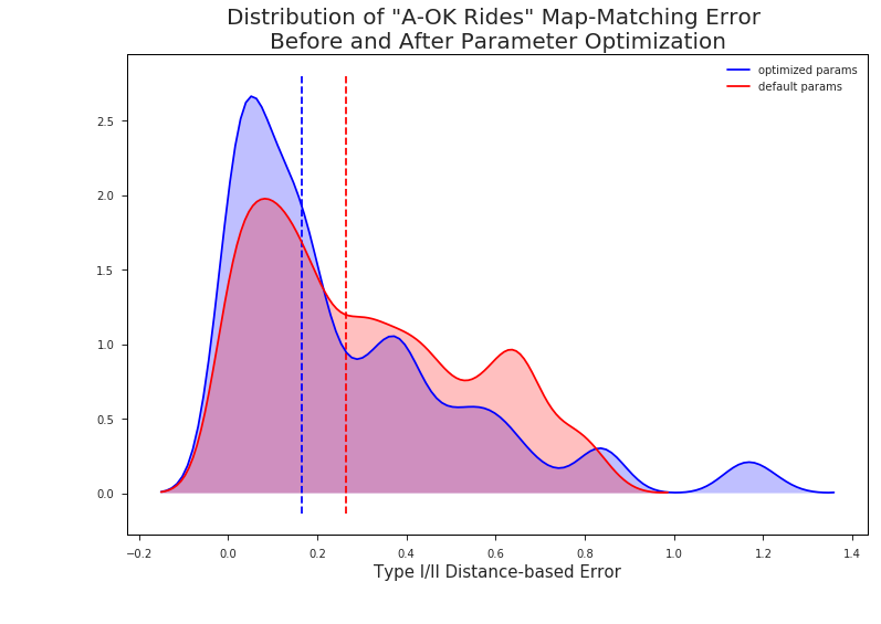
By tuning our map-matching parameters to fit the specific character of A-OK Rides’ data, we were able to reduce our median error rate from 26% to 17%. Although it might not seem like much on the chart, a 9% gain in median match accuracy can still have a huge impact on the overall performance of a near-real-time traffic platform like Open Traffic.
Most importantly, however, we’ve shown that we have a reliable methodology for fine-tuning our map-matching service to meet the specific needs of our data providers, whoever—and wherever—they may be.
